On Oct 4, 2003, the online version of the Decatur Herald & Review had a quote from Matt Vanover, spokesperson for the Illinois Department of Transportion (IDOT), that said "What we know is that 92 percent of the time when a driver is belted, their child passengers are going to be restrained as well. When the driver is unbelted, those child passengers are only restrained 72 percent of the time." The IDOT website has information that in November 2001, 71.4% of Illinois drivers were safety belted.
A game is played where a person flips a coin. If it the coin lands tails, the person loses $5. If the coin lands heads, then the person rolls a die. The person wins the last digit of the square of the value showing on the die (example: roll a 4, 4*4=16, so the person wins $6).
Create a probability distribution for the winnings of the game.
| Winnings | -5 | 1 | 4 | 5 | 6 | 9 | Total |
|---|---|---|---|---|---|---|---|
| Probability |
Find the mean and standard deviation for the amount of money won for this game.
Kerry Wood is the ace of the Chicago Cubs. During the regular season, he won 43.75% of the games that he started. Assume this rate continues during the post-season and that Kerry will start 6 games.
Try the problems before looking at the solutions.
The tree diagram can be constructed one of two ways. However, you only have the information to complete it for one of those ways.
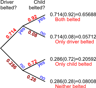
We know the answers to the second set of questions, so we'll start with the first event being whether or not the driver is belted and make the second event whether or not the child is belted. The tree diagram below answers the questions.

To help you understand the probabilities and the notations, here are the probabilities contained in the tree diagram above and how we found them.
Remember that the sum of the probabilities of all the outcomes must be one. For the tree diagram, that means that the sum of the probabilities on any set of branches must be 1. We'll use that to fill in the missing pieces of the puzzle. In the tree diagram above, the probabilities in light red were given in the problem and the probabilities in dark red were found by subtracting the given probabilities from 1.
P(driver belted) = 0.714 as given in story.
P(driver unbelted) = 1 - P(driver belted) = 1 - 0.714 = 0.286
The probabilities for the second event (the child being belted) are conditional probabilities. They are conditional upon whether or not the drive was belted.
P(child belted | driver belted) = 0.92 as given in story.
P(child unbelted | driver belted) = 1 - P(child belted | driver belted) = 1
- 0.92 = 0.08
P(child belted | driver unbelted) = 0.72 as given in story.
P(child unbelted | driver unbelted) = 1 - P(child belted | driver unbelted)
= 1 - 0.72 = 0.28
P(both belted) = P(driver belted and child belted) = 0.714 (0.92) = 0.65688
P(only driver belted) = P(driver belted and child unbelted) = 0.714(0.08) =
0.05712
P(only child belted) = P(driver unbelted and child belted) = 0.286(0.72) =
0.20592
P(neither belted) = P(driver unbelted and child unbelted) = 0.286(0.28) = 0.08008
The joint probability distribution is formed from the tree diagram. You multiply together the probabilities of each of the branches that you had to follow to get to the desired outcome.
| Child Belted | Child Unbelted | Total | |
|---|---|---|---|
| Driver Belted | 0.65688 | 0.05712 | 0.714 |
| Driver Unbelted | 0.20592 | 0.08008 | 0.286 |
| Total | 0.86280 | 0.13720 | 1.000 |
Okay, now the hard part is out of the way and you're ready to find the probabilities asked for in the problem.
This is a marginal probability, it makes absolutely no reference to the driver, so we take it from the total for the child belted column.
P(child belted) = 0.86280
The is a joint probability because of the word "and". We want both the driver to be belted and the child to be belted and we don't know anything ahead of time about the vehicle. This value comes from the inside portion of the table.
P(driver belted and child belted) = 0.65688
This is an "or" situation. We want either the driver to be belted or the child to be belted or both. We add the probability of the driver being belted and the probablity of the child being belted together, but in that number, we've counted those cases where both the driver and child were both belted. Since we don't want to double count those cases, we subtract the joint probability where both are belted.
P(driver belted or child belted) = P(driver belted) + P(child belted) - P(both
belted)
P(driver belted or child belted) = 0.714 + 0.8628 - 0.65688 = 0.91992
There is another way to tackle this problem. The driver being belted or the child being belted is the complement of neither one being belted. To use a complement, we take the part we don't want away from 1 to find the part we do want.
P(driver belted or child belted) = 1 - P(neither belted) = 1 - 0.08008 = 0.91992
This is a conditional probability. We know that the child is restrained (belted), we're looking for the probability that the driver is unbelted. We limit our view to just that part where the child is belted and then figure out what part of that is where the driver is unbelted.
The probability of a child being belted is 0.8628. Of that 0.8628, 0.20592 is where the driver was unbelted.
P(driver unbelted | child belted) = P(driver unbelted and child belted) /
P(child belted)
P(driver unbelted | child belted) = 0.20592 / 0.8628 = 0.23866
This is another conditional probability like the last question. However, in this case, we know that the child is unbelted, so we limit ourselves to the 0.1372 proportion of the cases where this happens. Of that 0.1372 where the child is unbelted, 0.05712 were with belted drivers.
P(driver belted | child unbelted) = 0.05712 / 0.1372 = 0.41633
If the flipped coin lands tails, you lose $5. This will happen 1/2 of the time, so the probability of winning -$5 is 1/2. If you flip the tail, the game is over, you don't even consider a the die. Here's what we have so far.
| Winnings | -5 | 1 | 4 | 5 | 6 | 9 | Total |
|---|---|---|---|---|---|---|---|
| Probability | 1/2 | 1 |
Okay, now for the roll of the die.
The values you can roll are 1, 2, 3, 4, 5, 6. The squares of those numbers are 1, 4, 9, 16, 25, and 36. The last digit of each of those is 1, 4, 9, 6, 5, 6.
If we flipped a head, then the probability of winning $1 is 1/6. But notice this is a conditional probability. It's conditional on the fact that we flipped a head in the first place and the chance of that happening is 1/2. The multiplication rule says we should multiply those two probabilities together to get the probability of both happening.
P(head and $1) = P(head) * P($1 | head) = 1/2 * 1/6 = 1/12
Likewise, the probabilities of winning $4, $5, or $9 is also 1/12. But the $6 winnings are twice as likely to occur since the 6 appeared as the last digit twice. So the probability of winning $6 is 2/12.
Since it appears that 12 is the common denominator, I'll change the 1/2 chance of losing $5 into 6/12 and write the probability distribution.
| Winnings | -5 | 1 | 4 | 5 | 6 | 9 | Total |
|---|---|---|---|---|---|---|---|
| Probability | 6/12 | 1/12 | 1/12 | 1/12 | 2/12 | 1/12 | 1 |
The mean is found by multiplying each value by its probability and adding.
The variance is found by multiplying the square of each value by its probability and adding and then subtracting the square of the mean from that sum.
I suggest adding two rows to the probability distribution
| x | -5 | 1 | 4 | 5 | 6 | 9 | Total |
|---|---|---|---|---|---|---|---|
| p(x) | 6/12 | 1/12 | 1/12 | 1/12 | 2/12 | 1/12 | 1 |
| x p(x) | -30/12 | 1/12 | 4/12 | 5/12 | 12/12 | 9/12 | 1/12 |
| x2 p(x) | 150/12 | 1/12 | 16/12 | 25/12 | 72/12 | 81/12 | 357/12 |
The mean is the sum of the "x p(x)" row or 1/12. So, your winnings are approximately $0.0833 or 8.33 cents per game played.
The variance is the sum of the "x2 p(x)" row minus the mean squared. That is 357/12 - (1/12)2 ≈ 29.743.
The standard deviation is the square root of the variance, so the sqrt(29.743) ≈ $5.454.
The first thing to realize is that this meets the criteria of a binomial experiment.
Now that we've established it satisifies the conditions of a binomial experiment, we can go about creating a probability distribution for it.
Label one column as x and another as p.
In the x column, put the values 0, 1, 2, 3, 4, 5, and 6. Those are the different possibilities for the number of games he can win in the six post-season starts.
Go to Calc / Probability Distributions / Binomial. Click the Probability radio button. Enter 6 for the number of trials and 0.4375 for the probability of success. The input column is x and the storage column is p. Click OK.
| x | 0 | 1 | 2 | 3 | 4 | 5 | 6 | Total |
|---|---|---|---|---|---|---|---|---|
| p(x) | 0.031676 | 0.147823 | 0.287434 | 0.298079 | 0.173880 | 0.054096 | 0.007012 | 1 |
P(At least 4 games) = P(4, 5, or 6 games). Since those are mutually exclusive, you can just add the probabilities together.
P(4) + P(5) + P(6) = 0.173880 + 0.054096 + 0.007012 = 0.234988
P(6) = 0.007012
P(No more than 2 games) = P(0, 1, or 2 games). Add those probabilities together.
P(0) + P(1) + P(2) = 0.031676 + 0.147823 + 0.287434 = 0.466933
P(3) = 0.298079
The number of trials is n = 32. The probability of success on a single trial is p = 0.4375. The probability of failure on a single trial is q = 0.5625. Remember that p and q have to add to be one.
The mean of a binomial distribution is the number of trials times the probability of success on a single trial.
Mean = μ = n p = 32 (0.4375) = 14
The variance is the product of the number of trials, the probability of success on a single trial, and the probability of failure on a single trial.
Variance = σ2 = n p q = 32 (0.4375) (0.5625) = 7.875
The standard deviation is the square root of the variance.
St. Dev = σ = sqrt(7.875) ≈ 2.806
Don't round these if they don't come out exact. Means and standard deviations do not have to be whole numbers.
The mean number of games you would expect Kerry to win is 14 games and the standard deviation for the number of games is 2.806.