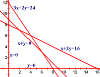
 The first step is to sketch the lines that correspond to the boundaries of the regions. These are found by replacing the ≤ and ≥ inequalities by an equal sign, =.
As a reminder, here is the linear programming problem we're working with.
| Maximize | P | = | 40x | + | 30y | ||
|---|---|---|---|---|---|---|---|
| Subject to: | x | + | 2y | ≤ | 16 | ||
| x | + | y | ≤ | 9 | |||
| 3x | + | 2y | ≤ | 24 | |||
| x | , | y | ≥ | 0 |
 The first step is to sketch the lines that correspond to the boundaries of the regions. These are found by replacing the ≤ and ≥ inequalities by an equal sign, =.
Do not place the objective function on the graph. We are graphing only the constraints or linear inequalities on this graph.
If you are graphing the functions by hand, putting the inequalities into standard form, Ax + By = C, for a line and then finding the x and y intercepts is probably the quickest way to graph it. If you want to graph them using technology, then solving them explicitly for y so they are in slope intercept form is probably the easiest method.
The graph of this is shown to the right.
Watch the Flash video: How to graph lines using Winplot [2.1 MB].
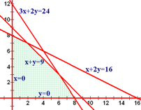
 Shading an inequality results in shading a half-plane. For most of the inequalities that we have from linear programming problems, it's pretty easy to tell which direction to shade just by looking at the inequality. When written in standard form Ax + By ≤ C or Ax + By ≥ C, then you will shade below or to the left for a less than or equal to or above or to the right for a greater than or equal to inequality.
That logic doesn't work if A or B is negative, though. For example, -3x + 2y ≤ -2 gets shaded to the right (below) the line while 3x - 2y ≤ 4 gets shaded to the left (above) the line. The sure fire way to tell which direction to shade is by picking a test point that is not on the boundary line and plugging that value into the inequality. The origin (0,0) is usually an easy point to use as long as it's not a solution to the linear equation. In our examples above, the left side of -3x + 2y ≤ -2 becomes -3(0) + 2(0) = 0, which is not less than -2, so the point (0,0) is not a solution to the linear inequality. Since (0,0) is above the line and doesn't work, we shade below the line.
The solution to the system of linear inequalities is the region that satisifies all of the inequalities and is called the feasible region.
Watch the Flash video: How to shade inequalities using Winplot [1.1 MB].
That feasible region is pretty big. There are an infinite number of points in the region where there could be a solution. The points (0,0), (0,1), (0,2), (1,2), (1,7), (2.16,4.92), etc., are all in the feasible region. Luckily, we have the fundamental theorem of linear programming to help.
The fundamental theorem of linear programming says that if there is a solution to a linear programming problem then it will occur at one or more corner points or the boundary between two corner points.
In other words, the solution is going to be on the edge of the region, not in the middle. A corner point is a vertex of the feasible region, so we need to figure out where those are.