 Bounded Feasible Regions
 It turns out that the slope of the objective function is very much related to the solution to a linear programming problem.
The first indication of this may have been with that last maximization problem where P = 30x + 30y. If you were to find the slope of that line, you would get m = -1. The line segment x + y = 9 also has a slope of m = -1. Intelligent minds go hmmmmm.
In case you don't remember, when a line is in standard form like P = Ax + By, the slope is -A/B.
The graph of the profit function is called an iso-profit line. It is called this because "iso" means "same" or "equal" and the profit anywhere on the line is the same.
When you watch this video, you will see iso-profit lines with different slopes sweeping across the feasible region starting at the origin and going as far as they can before leaving the feasible region. The further from line moves from the origin, the larger the profit becomes.
Watch the video and pay careful attention to where the maximum value of the objective function occurs and the slope of the edges of the feasible region.
Here are some points that you should get from the video. These are narrated in the video, but you may not have the ability to listen to them.
Watch the Flash video: Understanding the relationship between the slope of the objective function and the solution of a linear programming problem [2.7 MB].
Did you notice what the relationship between the slope and where the iso-profit line left the feasible region?
The slope of the objective function determines which corner point will be reached last. It can be summarized in this table.
| Corner Point | (8,0) | edge | (6,3) | edge | (2,7) | edge | (0,8) |
|---|---|---|---|---|---|---|---|
| Slope of Objective | less than -3/2 | -3/2 | between -3/2 and -1 | -1 | between -1 and -1/2 | -1/2 | greater than -1/2 |
The original problem was
| Maximize | P | = | 40x | + | 30y | ||
|---|---|---|---|---|---|---|---|
| Subject to: | x | + | 2y | ≤ | 16 | ||
| x | + | y | ≤ | 9 | |||
| 3x | + | 2y | ≤ | 24 | |||
| x | , | y | ≥ | 0 |
The objective function is P = 40x + 30y, which has a slope of -4/3.
The slope of -4/3 = -1.33333 falls between -3/2 and -1, so the optimal solution would be at the point (6,3).
Then, to find out what the maximum value is, we still need to plug x = 6 and y = 3 back into the objective function. P = 40(6) + 30(3) = 240 + 90 = 330.
The maximum value is P = 330 when x = 6 and y = 3.
 Bounded Feasible Regions
 A bounded feasible region may be enclosed in a circle.
A bounded feasible region will have both a maximum value and a minimum value for the objective function.
Why? Remember that the iso-profit line increases in value (assuming the coefficients are positive) as it moves through the feasible region. Since the feasible region is bounded, there is a limit on how far the iso-profit line can move. Therefore, there is a limit on how big it can get and there is a maximum value.
Moving the iso-profit towards the origin reduces the value of the objective function, but you can't go past the origin, so the value is bounded below and so there is a minimum.
There is a maximum and minimum value even if the objective function doesn't have positive coefficients, it's just not as well behaved.
Bounded feasible regions often result from standard maximum problems.
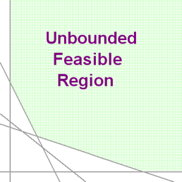
 Unbounded Feasible Regions
 An unbounded feasible region can not be enclosed in a circle, no matter how big the circle is.
If the coefficients on the objective function are all positive, then an unbounded feasible region will have a minimum but no maximum.
Why? Remember that the iso-profit line increases in value (assuming the coefficients are positive) as it moves through the feasible region. Since the feasible region is unbounded, there is nolimit on how far the iso-profit line can move. Therefore, there is no limit on how big it can get and there is no maximum value.
Moving the iso-profit line down and to the left towards the origin reduces the value of the objective function. In this case, there are boundary lines that block how far down or to the left you can go, so there is a minimum value that can be reached and still stay in the feasible region.
Unbounded feasible regions often result from standard minimization problems.
If the feasible region is empty, then there is no maximum or minimum values.
An empty region results when there are no points that satisfy all of the constraints. If there are no points that satisfy the constraints, there can be no points to have a maximum or minimum value.