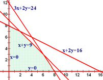
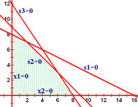
Let's take our linear programming problem and work with it.
| Maximize | P | = | 40x | + | 30y | ||
|---|---|---|---|---|---|---|---|
| Subject to: | x | + | 2y | ≤ | 16 | ||
| x | + | y | ≤ | 9 | |||
| 3x | + | 2y | ≤ | 24 | |||
| x | , | y | ≥ | 0 |
As mentioned earlier, we're going to switch from x and y to x1 and x2. The subscripted variables can be a little confusing at first, but they will make life much, much easier later on.
| Maximize | P | = | 40x1 | + | 30x2 | ||
|---|---|---|---|---|---|---|---|
| Subject to: | x1 | + | 2x2 | ≤ | 16 | ||
| x1 | + | x2 | ≤ | 9 | |||
| 3x1 | + | 2x2 | ≤ | 24 | |||
| x1 | , | x2 | ≥ | 0 |
We need to change the inequalities into equalities. This involves adding a variable to take up the slack between less than and equal to in the case of a ≤ constraint and subtracting a variable to remove the surplus in the case of a ≥ constraint.
The slack and surplus variables get subscripts as well. Use a subscript that corresponds to the constraint number. That is, use 1 for the first constraint, 2 for the second constraint, and so on.
We'll also require each of the slack and surplus variables to non-negative as well. In fact, every variable with the exception of the objective function will be required to be non-negative.
| Maximize | P | = | 40x1 | + | 30x2 | ||||||||
|---|---|---|---|---|---|---|---|---|---|---|---|---|---|
| Subject to: | x1 | + | 2x2 | + | s1 | = | 16 | ||||||
| x1 | + | x2 | + | s2 | = | 9 | |||||||
| 3x1 | + | 2x2 | + | s3 | = | 24 | |||||||
| x1 | , | x2 | , | s1 | , | s2 | , | s3 | ≥ | 0 |
Each of the lines can be identified by setting exactly one variable to zero.
| x1 | + | 2x2 | = | 16 | can be written as | s1 | = | 0 |
| x1 | + | x2 | = | 9 | can be written as | s2 | = | 0 |
| 3x1 | + | 2x2 | = | 24 | can be written as | s3 | = | 0 |
| x1 | = | 0 | can be written as | x1 | = | 0 | ||
| x2 | = | 0 | can be written as | x2 | = | 0 |
Here is the feasible region shown in two ways. The first way we saw earlier when lines were identified by x and y. Now we see them identified by a single variable equaling zero.


Each line can be identified by one variable, the one variable that is set equal to zero. Since that variable is always zero on that line, it is called non-basic. Think of "basic" as meaning elementary, foundational, or important. Since that variable is zero, it's not important, or non-basic.
Since each line is identified by one variable, the non-basic variable, being zero, each intersection point can be identified by two variables being zero. The two variables that are zero at an intersection point correspond to the non-basic variables and the other variables are basic variables.
That means that is is possible to find the coordinates of all the points on the graph by creating a table listing all the different combinations of variables where exactly two of them at a time are zero. The two variables that are zero are the non-basic variables and the rest of the variables are basic.
| Pt | x1 | x2 | s1 | s2 | s3 |
|---|---|---|---|---|---|
| A | 0 | 0 | |||
| B | 0 | 0 | |||
| C | 0 | 0 | |||
| D | 0 | 0 | |||
| E | 0 | 0 | |||
| F | 0 | 0 | |||
| G | 0 | 0 | |||
| H | 0 | 0 | |||
| I | 0 | 0 | |||
| J | 0 | 0 |
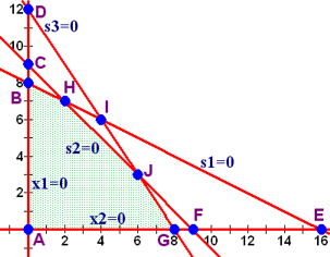
The figure shows where each of those points is on the graph.
The key now is to figure out what the rest of the variables are. You need to find x1 and x2 to do that.
Take the values you know and plug them into the system of equations. Then solve for the remaining variables.
| 0 | + | 0 | + | s1 | = | 16 | ||||
| 0 | + | 0 | + | s2 | = | 9 | ||||
| 0 | + | 0 | + | s3 | = | 24 |
So s1 = 16, s2 = 9, and s3 = 24
Since x1 and s1 are both in the first equation, plug zero in for them to find x2. When you do that, you get 2x2 = 16 so x2 = 8.
Now plug the x1 = 0 and x2 = 8 into the other equations to find s2 and s3.
| 0 | + | 8 | + | s2 | = | 9 | ||||
| 0 | + | 8 | + | s3 | = | 24 |
So x2 = 8, s2 = 1, and s3 = 16
Since x2 and s3 are both in the third equation, plug zero in for them to find x1. When you do that, you get 3x1 = 24 so x1 = 8.
Now plug the x1 = 8 and x2 = 0 into the other equations to find s1 and s2.
| 8 | + | 0 | + | s1 | = | 16 | ||||
| 8 | + | 0 | + | s2 | = | 9 |
So x1 = 8, s1 = 8, and s2 = 1
Since s1 and s2 are in the first and second equations, plug zero in for them to find x1 and x2 . When you do that, you get a system of linear equations.
| x1 | + | 2x2 | = | 16 |
| x1 | + | x2 | = | 9 |
When you solve that system of linear equations (using substitution, elimination, Gaussian reduction, matrix inverses, or Cramer's Rule), you get x1 = 2 and x2 = 7. A refresher is avaliable about how to solve a system of linear equations.
Then, once you know x1 and x2, plug them into the third equation to find s3.
| 2 | + | 7 | + | s3 | = | 24 |
So x1 = 2, x2 = 7, and s3 = 15
| Pt | x1 | x2 | s1 | s2 | s3 |
|---|---|---|---|---|---|
| A | 0 | 0 | 16 | 9 | 24 |
| B | 0 | 8 | 0 | 1 | 16 |
| C | 0 | 9 | -2 | 0 | 6 |
| D | 0 | 12 | -8 | -3 | 0 |
| E | 16 | 0 | 0 | -7 | -24 |
| F | 9 | 0 | 7 | 0 | -3 |
| G | 8 | 0 | 8 | 1 | 0 |
| H | 2 | 7 | 0 | 0 | 15 |
| I | 4 | 6 | 0 | -1 | 0 |
| J | 6 | 3 | 4 | 0 | 0 |
From the graph that we had earlier, we can tell that points A, B, G, H, and J are feasible. Let's add another column to the table to identify whether or not the point is feasible.

| Pt | x1 | x2 | s1 | s2 | s3 | Feasible? |
|---|---|---|---|---|---|---|
| A | 0 | 0 | 16 | 9 | 24 | yes |
| B | 0 | 8 | 0 | 1 | 16 | yes |
| C | 0 | 9 | -2 | 0 | 6 | no |
| D | 0 | 12 | -8 | -3 | 0 | no |
| E | 16 | 0 | 0 | -7 | -24 | no |
| F | 9 | 0 | 7 | 0 | -3 | no |
| G | 8 | 0 | 8 | 1 | 0 | yes |
| H | 2 | 7 | 0 | 0 | 15 | yes |
| I | 4 | 6 | 0 | -1 | 0 | no |
| J | 6 | 3 | 4 | 0 | 0 | yes |
Notice anything about the points that are not feasible?
What if I mention that one of the restrictions was that every variable be non-negative? Ahh, if there is any negative, then the point is not feasible. Wow, that's cool.
Let's add one more column, this time for the objective function. But we only need to evaluate it for those points that are in the feasible region.
| Pt | x1 | x2 | s1 | s2 | s3 | Feasible? | P = 40x1 + 30x2 |
|---|---|---|---|---|---|---|---|
| A | 0 | 0 | 16 | 9 | 24 | yes | 0 |
| B | 0 | 8 | 0 | 1 | 16 | yes | 240 |
| C | 0 | 9 | -2 | 0 | 6 | no | N/A |
| D | 0 | 12 | -8 | -3 | 0 | no | N/A |
| E | 16 | 0 | 0 | -7 | -24 | no | N/A |
| F | 9 | 0 | 7 | 0 | -3 | no | N/A |
| G | 8 | 0 | 8 | 1 | 0 | yes | 320 |
| H | 2 | 7 | 0 | 0 | 15 | yes | 290 |
| I | 4 | 6 | 0 | -1 | 0 | no | N/A |
| J | 6 | 3 | 4 | 0 | 0 | yes | 330 |
The largest value of the objective function is P = 330 and occurs when x1 = 6 and x2 = 3.
We now have the ability to complete the entire linear programming problem without making a graph at all. Woohoo!