Normal Probabilities
I.Q. scores are normally distributed with a mean of 100 and a standard deviation
of 15. Use simulation to find the probability that an individual will have an
I.Q. of ...
- greater than 130,
- less than or equal to 80, or
- between 90 and 110
Sure, there are tables you can look this kind of thing up in, but that would
defeat the purpose of simulation. Simulation also helps the students to understand
where the numbers in the table come from.
The Problem
The main problem in this simulation is getting a list of normally distributed
numbers. The random number generators with most programs are uniform generators
only. We are going to use a computer algebra system (CAS) to generate the list
of numbers and answer the probabilities for us.
Type of Simulation
Since we are looking for a probability, this is a case where we will simulate
numbers and then classify them as success or failure and take the number of
successes divided by the number of trials to get the relative frequency or empirical
probability.
In this case, the simulation is easy. We just have to generate one number.
Either it is in the interval we're trying to find the probability of or it isn't
in the interval. If it is in the interval, we'll call it a success and if it
isn't, we'll call it a failure. We will generate lots and lots of numbers, because
the more numbers we generate, the more accurate our probability will be.
The Simulation
The computer algebra system that you use is really up to you, but I would recommend
using one that you have instead of one that you don't have. I'll show some instructions
for Maple and Derive and if you have Mathematica, then hopefully you'll be able
to figure it out from the examples shown.
Derive
Derive has a function called random_normal(s,m) that will
generate a random number with a mean of m and a standard deviation of s. To
generate a single random number from our I.Q. problem, we would use random_normal(15,100).
We can then use the if(condition,true,false) statement to
see if it satisfies what we're looking for. We'll return 1 if the statement
is true and 0 if false and that way we can add teh values we'll have the number
of successes.
prob1(n) := sum(IF(RANDOM_NORMAL(15, 100) > 130, 1, 0), i, 1, n)/n
The function above will randomly generate n normally distributed numbers with
a mean of 100 and standard deviation of 15, count how many are are greater than
130, and return the value as a probability.
To execute the statement, type prob1(1000) and then hit the approximate
button. Do this a couple of times and get answers like 0.026, 0.019, or 0.024.
The theoretical value is 0.0228, so not too bad.
Now, try prob1(10000) and you get 0. Hmm, obviously something
is wrong. We should get a more accurate answer, not a useless one. It turns
out that the function has problems if you use over 1001 values. Don't know why,
but it does. Just be careful and don't believe everything a computer algebra
system tells you.
Similarly, to find the second probability, we could define
prob2(n) := sum(IF(RANDOM_NORMAL(15, 100) <= 80, 1, 0), i, 1, n)/n
and then find prob2(1000) a couple of times and get answers like
0.099, 0.088, and 0.091. The theoretical value is approximately 0.0918, so again,
in the ballpark.
To find the third probability, we have a slight problem. We have a between
condition, meaning that the random number must be between two numbers. If we
try something like
prob3(n) := sum(IF(RANDOM_NORMAL(15, 100) > 90 AND RANDOM_NORMAL(15,
100) < 110, 1, 0), i, 1, n)/n
we will run into problems. The problem is that it will actually generate two
random numbers and so the number we're testing to see if it's greater than 90
won't actually be the same number we're testing to see if it's less than 110.
Oops, big problem there.
The next part is really messy and you may want to just use the table in the
back of your Statistics text to answer the question. You can define a program
in Derive to find the probability.
prob3(n) := PROG(s := 0, i := 0, LOOP(IF(i = n, RETURN 1·s/n),
x := RANDOM_NORMAL(15, 100), IF(x > 90 AND x < 110, s :+ 1), i :+ 1))
The advantage to this is that it doesn't have the limitations of the sum command
and can handle more than 1001 numbers. So, try prob3(10000) and
wait about 40 seconds (on a 350 MHz Pentium II computer) while it thinks about
it and finally comes up with 0.4947, 0.5027, or 0.4957. The theoretical answer
is approximately 0.4972, so once again, it's in the right area.
If you don't want to have Derive count the numbers and you want to do that
yourself, then you can use the vector command like this:
normlist(n) := VECTOR(RANDOM_NORMAL(15, 100), x, n)
This will generate n random numbers from a normal distribution with a mean
of 100 and a standard deviation of 15. You can then go through and count how
many fall in the interval desired.
If you want to be really nice, then add the sort command to
that and Derive will put them in order for you.
normlist(n) := SORT(VECTOR(RANDOM_NORMAL(15, 100), x, n))
As an example,
normlist(10) = [75.53853769, 76.20925104, 82.00811444, 83.53464762, 83.63545252,
87.50281676, 91.07995753, 98.92183695, 99.74776046, 109.3756475] and
you can see that 4/10 of the numbers lie between 90 and 110, so the probability
would be 0.4.
One thing to remember with Derive is that you always need to use the Approximate
button instead of the simplify button. Either that or make sure your in approximate
mode instead of exact mode. Also, Derive doesn't have useful facilities for
generating histograms or other plots of the data, so the students won't be able
to visualize the normality of the data.
Maple 8
 Maple
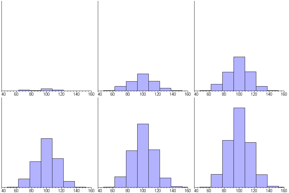
is quite a bit more powerful (and expensive) than Derive. The animated image
shows the generation of 1000 random numbers that are normally distributed with
a mean of 100 and a standard deviation of 15. Each frame in the animation includes
25 more samples than the previous frame. Each bar is one standard deviation
wide.
While this isn't exactly a simulation, it does show that the numbers you're
using in your simulation really do fit the normal distribution which can help
verify that the simulations you're peforming are accurate.
Here is the Maple code used to produce the animation.
> with(stats):
> with(random):
> with(plots):
> Digits:=5:
> data1:=[random[normald[100,15]](1000)]:
> classes:=[32.5..47.499, 47.50..62.499, 62.50..77.499, 77.50..92.499,
92.50..107.499, 107.50..122.499, 122.50..137.499, 137.50..152.499, 152.50..167.499]:
> display(seq(statplots[histogram](transform[tallyinto](data1[1..25*i],classes),
view=[40..160,0..30], tickmarks=[5,0]),i=1..40), insequence=true);
Return to Simulation Page
 Maple
is quite a bit more powerful (and expensive) than Derive. The animated image
shows the generation of 1000 random numbers that are normally distributed with
a mean of 100 and a standard deviation of 15. Each frame in the animation includes
25 more samples than the previous frame. Each bar is one standard deviation
wide.