Maxima doesn't have built in functions to perform the numeric approximations using the various methods. This supplement will supply functions that you can use to find the approximations. You can copy and paste this code into your code.
Note that there is no error checking done in the development portion of functions, so if you use them, be sure that \( n \) is an integer or that \( n \) is even in the case of Simpson's rule. There is error checking added to the combined functions at the end.
Each method is called with four parameters: the function, the left-most limit, the right-most limit, and the number of subintervals. method(f, a, b, n);
Each of the functions creates a step-size \( h = \Delta x = \dfrac{b-a}{n} \). We will also treat \( x_0 = a \) and \( x_n = b \).
For left-hand endpoints, we have \( x_k = a + (k-1) h \) for \( k = 1 \dots n \). Through reindexing \(i = k-1 \), we can simplify this to \( x_i = a + i h \) for \( i = 0 \dots n-1 \).
\(\displaystyle \int_a^b f(x) dx \approx h \sum\limits_{i=0}^{n-1} f(x_i) \)
lefthand(f,a,b,n):=block([h,i],
    h:(b-a)/n,
    h*float(sum(ev(f,x=a+i*h),i,0,n-1))
)$ For right-hand endpoints, we have \( x_k = a + k h \) for \( k = 1 \dots n \).
\(\displaystyle \int_a^b f(x) dx \approx h \sum\limits_{i=1}^{n} f(x_i) \)
righthand(f,a,b,n):=block([h,i],
    h:(b-a)/n,
    h*float(sum(ev(f,x=a+i*h),i,1,n))
)$ For midpoints, we have \( x_k = a + (k+0.5) h \) for \( k = 0 \dots n-1 \).
\( \displaystyle \int_a^b f(x) dx \approx h \sum\limits_{i=1}^{n} f(x_i) \)
midpoint(f,a,b,n):=block([h,i],
    h:(b-a)/n,
    h*float(sum(ev(f,x=a+(i+0.5)*h),i,0,n-1))
)$ \( \displaystyle \begin{align*} \int_a^b f(x) dx \approx & \frac h 2 \left [ f(x_0) + 2 f(x_1) + 2f(x_2) + \dots + 2 f(x_n) + 2 f(x_{n-1}) + f(x_n) \right ] \\ = & h \left [ \frac 1 2 \left [ f(x_0) + f(x_n) \right ] + f(x_1) + f(x_2) + \dots + f(x_n) + f(x_{n-1}) \right ] \\ = & h \left [ \frac { f(a) + f(b) }{2} + \sum\limits_{k=1}^{n-1} f(x_k) \right ] \end{align*} \)
trapezoid(f,a,b,n):=block([h,i],
    h:(b-a)/n,
    h*(float((ev(f,x=a)+ev(f,x=b))/2+sum(ev(f,x=a+i*h),i,1,n-1)))
)$ There is a requirement that \( n \) is even in this method.
\( \displaystyle \int_a^b f(x) dx \approx \frac h 3 \left [ f(x_0) + 4 f(x_1) + 2f(x_2) + \dots + 2 f(x_n) + 4 f(x_{n-1}) + f(x_n) \right ] \)
Okay, this one gets a little tricky.
We're going to group every pair of intervals together.
\( \displaystyle \int_a^b f(x) dx \approx \frac h 3 \left [ \underbrace{ f(x_0) + 4 f(x_1) + f(x_2) }_{k=1} + \underbrace{ f(x_20) + 4 f(x_3) + f(x_4) }_{k=2} + \dots + \underbrace{ f(x_{n-2}) + 4 f(x_{n-1}) + f(x_n) }_{k=n/2} \right ] \)
Let \( x_k = a + (2i-1)h \) where \( i = 1 \dots \frac n 2 \). This gives us the midpoint of each interval and then the left-endpoint is \( x_k - h \) and the right-endpoint is \( x_k + h \).
\( \displaystyle \int_a^b f(x) dx \approx \frac h 3 \left [ f(x_0) + 4 f(x_1) + 2f(x_2) + \dots + 2 f(x_n) + 4 f(x_{n-1}) + f(x_n) \right ] \)
simpson(f,a,b,n):=block([h,i],
    h:(b-a)/n,
    h/3*float(sum(ev(f,x=a+(2*i-2)*h)+4*ev(f,x=a+(2*i-1)*h)+ev(f,x=a+(2*i)*h),i,1,n/2))
)$ Here is code that you can copy all at once rather than having to copy five separate sections. However, you should copy just the portion you need.
This code includes error checking on \( n \).
lefthand(f,a,b,n):=block([h,i],
    if n > 0 and integerp(n) then (
        h:(b-a)/n,
        h*float(sum(ev(f,x=a+i*h),i,0,n-1))
    ) else error("The number of intervals must be a positive integer")
)$
righthand(f,a,b,n):=block([h,i],
    if n > 0 and integerp(n) then (
        h:(b-a)/n,
        h*float(sum(ev(f,x=a+i*h),i,1,n))
    ) else error("The number of intervals must be a positive integer")
)$
midpoint(f,a,b,n):=block([h,i],
    if n > 0 and integerp(n) then (
        h:(b-a)/n,
        h*float(sum(ev(f,x=a+(i+0.5)*h),i,0,n-1))
    ) else error("The number of intervals must be a positive integer")
)$
trapezoid(f,a,b,n):=block([h,i],
    if n > 0 and integerp(n) then (
        h:(b-a)/n,
        h*(float((ev(f,x=a)+ev(f,x=b))/2+sum(ev(f,x=a+i*h),i,1,n-1)))
    ) else error("The number of intervals must be a positive integer")
)$
simpson(f,a,b,n):=block([h,i],
    if n > 0 and evenp(n) then (
        h:(b-a)/n,
        h/3*float(sum(ev(f,x=a+(2*i-2)*h)+4*ev(f,x=a+(2*i-1)*h)+ev(f,x=a+(2*i)*h),i,1,n/2))
    )
    else error ("The number of intervals must be an even positive integer")
)$Begin by copying the code above into your Maxima file and then executing it before you try to use it.
Let's say that you have \( \displaystyle \int_1^4 \exp \left (-\frac 1 3 x^4 \right ) dx \) and you want to find the approximations with 10 sub-intervals. You could use this code to obtain the results.
f:exp(-1/3*x^4)$
a:1$
b:4$
n:10$
lefthand(f,a,b,n);
righthand(f,a,b,n);
midpoint(f,a,b,n);
trapezoid(f,a,b,n);
simpson(f,a,b,n);
romberg(f,x,a,b);
The romberg() function at the end returns what we'll consider to be the correct answer. Also note that you could have hard-coded the values, which is okay for a one-time deal, but if you want to repeat the process with different values of \( n \), then this makes it easier as you only need to change one value.
The romberg() function sometimes fails to return a correct answer and its accuracy is not as great as some of the other methods. The quad_qags() function is an alternative, but it returns a list of four values: The first component of quad_qags() is the answer, the second is an approximate error, the third is the number of iterations, and the last is an error code where 0 means there were no problems. You can add a [1] to the end of the quad_quags() function to get just the approximation.
| Method | Command | Result | Absolute Error |
|---|---|---|---|
| Integrate | integrate(exp(-1/3*x^4),x,1,4); |
\( \displaystyle \frac{{{3}^{\frac{1}{4}}}\,\left( \operatorname{gamma\_ incomplete}\left( \frac{1}{4},\frac{1}{3}\right) -\operatorname{gamma\_ incomplete}\left( \frac{1}{4},\frac{256}{3}\right) \right) }{4} \) | 0 |
| Left Hand | lefthand(exp(-1/3*x^4),1,4,10); |
0.368522855082048 | 0.1146901479661376 |
| Right Hand | righthand(exp(-1/3*x^4),1,4,10); |
0.1535634619099112 | 0.1002692452059991 |
| Midpoint | midpoint(exp(-1/3*x^4),1,4,10); |
0.2502105824409427 | 0.003622124674967586 |
| Trapezoid | trapezoid(exp(-1/3*x^4),1,4,10); |
0.2610431584959796 | 0.00721045138006926 |
| Simpson | simpson(exp(-1/3*x^4),1,4,10); |
0.2538171155585557 | 1.55915573546439×10⁻⁵ |
| Romberg | romberg(exp(-1/3*x^4),x,1,4); |
0.2538321895064358 | 5.176094745040771×10⁻⁷ |
| Quad Qags | quad_qags(exp(-1/3*x^4),x,1,4); |
[ 0.2538327071159103, 5.84575770053847×10⁻¹², 63, 0 ] | 5.551115123125783×10⁻¹⁷ |
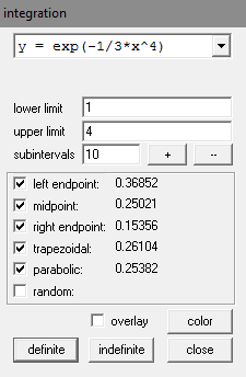
Winplot has the ability to perform numeric integration as well. After creating your explicit function, go to One > Measurement > Integrate f(x) dx. After putting in the values and choosing the methods to use, click the definite button to get the approximations.

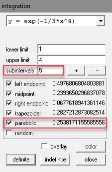
Note that Simpson's method is actually called parabolic and that definition of a subinterval is different than what we have been using. In Winplot, the number of subintervals (10 in this example) refers to the number of parabolas, not the number of subintervals. Because we paired the intervals together to form parabolas, the 10 subintervals uses 5 parabolas.
To get the same number we obtained, you would need to put in 5 for the number of subintervals (parabolas), but then the other values wouldn't match what we have. Before you say that is what we have, notice that Winplot only gives 5 decimal places in the approximation. You can change the number of decimal places in the answer by going to Misc > Settings > miscellany.
Changing output to 16 decimal places and the number of parabolas (subintervals) to 5, we get the same value we had before.
