Minitab Notes for Activity 1

You do not need to print out any of the graphs that you generate for this activity. Just look at them on the screen and answer questions based off of them in the activity. There is one graph (the histogram) that you need to copy onto your paper.

Creating the Worksheet

This step can be skipped if you go to File / Open Worksheet and open the walk.mtw file the instructor created for you. This section is still good reading for you to learn about creating worksheets, though.

Make Patterned Data There is a little bit of setup that you need to do before entering the data. Minitab can also help by creating some of the values for you.

Label the columns as team, heat, and time.
Have Minitab automatically enter the team data for you.
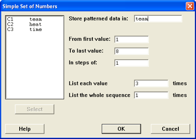
1. Choose Calc / Make Patterned Data / Simple Set of Numbers
2. For the team column, the values go from 1 to the number of teams (shown as 8 in the figure) and each value should be repeated 3 times since there are 3 heats for each team.
3. Click OK
Have Minitab automatically enter the heat data for you.
1. Choose Calc / Make Patterned Data / Simple Set of Numbers
2. For the heat column, the values go from 1 to 3 since there are 3 heats for each team. Each value is listed only once, but the whole sequence is repeated for each team (8 in our example).
3. Click OK
Enter the time data yourself
Save the Project
1. Choose File / Save Project As
2. Change to the R: drive and into the proper folder for your section (01, 02, or 03).
3. Change into the act1 folder
4. Type a file name that is unique to your group.
5. Click Save

Summarizing the Data (Question 4)

Once you have your data entered into Minitab, you may work with it. One of the most common things we will do is display the descriptive statistics. This screen will give you the following statistics by default.

N = Sample Size
N* = Number of missing cases
Mean = Mean
SE Mean = Standard Error of the Mean
StDev = Standard Deviation
Minimum = Minimum
Q1 = 1st Quartile
Median = Median
Q3 = 3rd Quartile
Maximum = Maximum value

You can change the statistics that are given by clicking on the statistics button. In particular, the N* and SE Mean won't be used right now. The SE Mean will be used in later chapters, but the number of missing cases is rarely used. Other options in the statistics menu that we will use occasionally are the variance, range, interquartile range, and sum of squares.

You may describe more than one variable at a time. However, in this problem, we only have one variable, time, that we want to describe. The other two variables are categorical variables used for classification purposes only, it would make no sense to describe them. Sample output from the descriptive statistics command is shown in the figure.

Using All of the Data

This is the way to describe the time for all of the teams and all of the heats.

Go to Stat / Basic Statistics / Display Descriptive Statistics
Select the time column for the variables section
Click OK

You should get some output that looks something like this.

Descriptive Statistics: time
Variable   N  N*   Mean  SE Mean  StDev  Minimum     Q1  Median     Q3  Maximum
time      24   0  20.75     1.09   5.32    10.76  17.79   19.99  23.90    33.96

Grouping the Data by Another Variable

Descriptive Statistics by a categorical variable This is the way to describe the time for each of the heats. We use the "By Variable" option to do this. The column used for the By Variable should be a categorical variable such as the gender, race, age group (but not age as a number), or heat number. There should be few categories for this variable, do not use variables that have large numbers of unique values for the By Variable. Do not use measurement variables (height, weight, age, time) as the by variable.

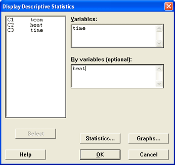
Go to Stat / Basic Statistics / Display Descriptive Statistics
Select the time column for the variables section
Check the By Variable box
Tell Minitab to describe the data by the variable heat.
(Optional) Click on Graphs and turn on the Graphical Summary.
Click OK

Box Plots (Question 5e)

Adding Mean Symbol for step 3 A box plot is a way to graphically explore the data. Choose the variable you want to describe as the y variable and the way you want to group the data by the classification variable x. The box plot does not normally have the mean on it, but we will add it here for reference purposes.

Go to Graph / Boxplot
You have four choices for the type of box plot to make.
1. One Y - Simple: Use this when you have just a single column of data and want just one box plot.
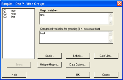
2. One Y - With groups: Use this when you have two columns, one that contains the data (like the time) and another that contains a classification variable (like the heat or team number). This will generate multiple side-by-side graphs. This is the one that we want in this problem.
3. Multiple Y's - Simple: Use this when you have two or more columns that contain the data. This could be used when you have two pieces of information about each of the cases. For example, if you wanted to make a box plot of the height and weight of people.
4. Multiple Y's - With groups: Use this when you have two or more columns of data and you have a classification variable to further group the data. For example, if you want the height and weight of people broken down by their gender, then you would select this option.
Select time as the Y variable and heat as the X variable.
Although not a necessary part of the box plot, we're going to add a symbol for the mean to the graph. Click on the Data View button.
1. Click on the checkbox for the Mean Symbol
2. Optional: If you will click on the Categorical variables for attribute assignment and select the heat variable, then it will color code the graphs and provide a key for you.
3. Click OK to return to the box plot menu
Click OK

Histograms (Question 6)

Default histogram before changing settings A histogram is a good way to look the data and see where it lies. We can also use it to let Minitab count the number in each group for us, rather than us having to do it manually.

Normally, we would let Minitab just automatically assign groups for us, but in this case, we're specifically looking for bars that are one standard deviation wide. That means that we're going to have to do some extra work that we wouldn't normally have to do.

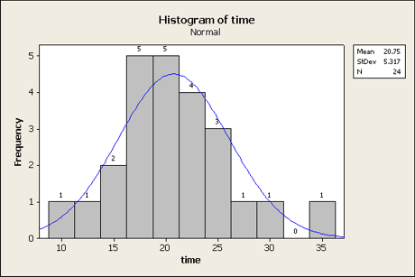
For this example, let's assume that the mean is 20.75 and the standard deviation is 5.32. Find the mean minus three times the standard deviation and the mean plus three times the standard deviation: 20.75 - 3(5.32) = 4.79 and 20.75 + 3(5.32) = 36.71. These numbers correspond to our lowest and highest class boundaries and will be used later.

Go to Graph / Histogram
You have choices for the type of histogram that you want. Most of the time, we will use the simple one or the with fit graph. The fit tries to fit a normal distribution to the data and can be useful for determining whether or not the data comes from a normally distributed population. This is addressed in this unit but it becomes very important later on in the book. Go ahead and choose the with fit for now.
Select time as the graph variable
Click on Labels
1. Under Title / Footnotes, you can add text to describe the graph.
2. Under Data Labels, Check the use y-value labels radio button so that it will label the graph with the frequency of each bar.
Click OK to generate the histogram.

Modified histogram The old version of Minitab would allow you to set all kinds of options before you generated the graph. The new version allows you to look at the graph and then play with the settings. There's arguments in favor of both directions, but for most people, the new way is probably better. The rest of this will involve changing the graph to give us what we want to have.

Position the cursor over the bars and then right click the mouse button the graph and choose "Edit Bars" (or hit control-T)
(Optional: Recommended) Under the Attributes menu, you can make the following changes to format the bars of the histogram. By default, the bars are not shaded, so it can be difficult to see them. You can change that by following these steps.
1. For the Fill pattern, click Custom
2. Change the type (I like the right slant)
3. Change the color (or use automatic)
Click on the Binning tab
1. Change the interval type to Cutpoint
2. Select "Midpoint/Cutpoint positions"
3. In the positions box, enter something like the following (without quotes) "4.79:36.71/5.32". That notation is the minimum : maximum / width (but without spaces). You could alternatively enter the boundary for each bar and separate them by spaces. Use your data, not the 4.79:36.71/5.32, that is only for the example here in the instructions.

Save Your Work (optional)

Since the file "walk.mtw" was already provided for you, you will probably be okay without saving a project file for this activity. There's not much work that wouldn't be easy to recreate if you messed up and had to go back.

Be sure to save your work! This allows you to go through and work on the activity incrementally (you can do part of it one day and finish it another day). All open windows are saved when you save the project, but if you close a graph, it won't be saved. When you are completely done with the project, you may wish to close the graphs. This will make the files smaller and keep us from running out of room on the drive.