Independent variables can be combined to form new variables. The mean and variance of the combination can be found from the means and the variances of the original variables.
| Combination of Variables | In English (Melodic Mathematics) |
| The mean of a sum is the sum of the means. | |
| The mean of a difference is the difference of the means. | |
| The variance of a sum is the sum of the variances. | |
| The variance of a difference is the sum of the variances. |
Since we are combining two variables by subtraction, the important rules from the table above are that the mean of the difference is the difference of the means and the variance of the difference is the sum of the variances.
It is important to note that the variance of the difference is the sum of the variances, not the standard deviation of the difference is the sum of the standard deviations. When we go to find the standard error, we must combine variances to do so. Also, you're probably wondering why the variance of the difference is the sum of the variances instead of the difference of the variances. Since the values are squared, the negative associated with the second variable becomes positive, and it becomes the sum of the variances. Also, variances can't be negative, and if you took the difference of the variances, it could be negative.
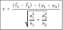
 When the population variances are known, the difference of
the means has a normal distribution. The variance of the
difference is the sum of the variances divided by the sample
sizes. This makes sense, hopefully, because according to the
central limit theorem, the variance of the sampling
distribution of the sample means is the variance divided by
the sample size, so what we are doing is add the variance of
each mean together. The test statistic is shown.
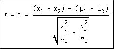
 When the population variances aren't known, the
difference of the means has a Student's t distribution.
However, if both sample sizes are large enough, then
you will be using the normal row from the t-table, so
your book lumps this under the normal distribution,
rather than the t-distribution. This gives us the chance to work the problem without knowing if
the population variances are equal or not. The test statistic is shown, and is identical to above,
except the sample variances are used instead of the population variances.
Ok, you're probably wondering how do you know if the variances are equal or not if you don't know what they are. Some books teach the F-test to test the equality of two variances, and if your book does that, then you should use the F-test to see. Other books (statisticians) argue that if you do the F-test first to see if the variances are equal, and then use the same level of significance to perform the t-test to test the difference of the means, that the overall level of significance isn't the same. So, the Bluman text tells the student whether or not the variances are equal and the Triola text makes the students test it for themselves.
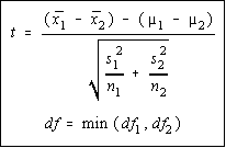
 Since you don't know the population variances, you're going
to be using a Student's t distribution. Since the variances are
unequal, there is no attempt made to average them together as
we will in the next situation. The degrees of freedom is the
smaller of the two degrees of freedom (n-1 for each). The
"min" function means take the minimum or smaller of the
two values. Otherwise, the formula is the same as we used
with large sample sizes.
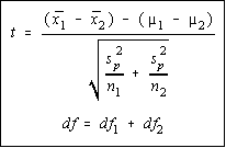
 If the variances are equal, then an effort is made to average them
together. Now, equal does not mean identical. It is possible for two
variances to be statistically equal but be numerically different. We
will find a pooled estimate of the variance which is simply the
weighted mean of the variance. The weighting factors are the degrees
of freedom.
 Once the pooled estimate of the variance is computed, this
mean (average) variance is used in the place of the individual
sample variances. Otherwise, the formula is the same as
before. The degrees of freedom are the sum of the individual
degrees of freedom.